Pipeline Pressure Drop Calculation – Darcy–Weisbach Equation & Excel Tutorial

This example shows that even modest pipe roughness can contribute significantly to pressure losses over long distances. An Excel spreadsheet can perform these calculations quickly for any combination of pipe sizes, flow rates and fluids.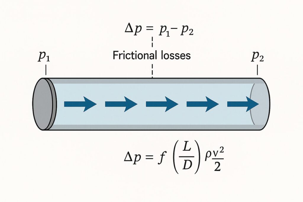

Professional insights for process and mechanical engineers

When designing or troubleshooting any fluid system—whether it’s an industrial water network, a chemical plant or a process pipeline—pressure drop is one of the first things engineers calculate. Excessive friction losses waste energy, increase operating costs and can lead to undersized equipment or process upsets. Accurately predicting how much pressure will be lost along a pipeline ensures the pump or compressor is sized correctly and that valves, instruments and downstream equipment all operate within their design envelopes.

In this article we explore the Darcy–Weisbach equation, the most widely accepted method for determining major pressure losses in pipes. We also show how to implement the calculation in an Excel spreadsheet and share tips on reducing pressure drop through better design. Throughout, the tone is professional and straightforward—suitable for engineers, managers and clients who need reliable calculations—and everything is optimised for search so it’s easy to find on today’s AI‑driven browsers.

Why pressure drop matters

Pipelines are rarely “frictionless.” As fluid flows through a pipe, the roughness of the internal surface and the turbulence of the flow cause resistance. That resistance manifests as a drop in pressure or, when expressed in terms of head, as a loss of energy. Pumps or compressors have to work harder to overcome that loss. If the pressure drop is underestimated, the system may not achieve the required flow; if it is overestimated, capital costs rise because equipment is oversized. A systematic calculation prevents these problems and provides a basis for optimisation.

The Darcy–Weisbach equation

The major pressure loss (or head loss) in a straight pipe due to friction can be calculated with the Darcy–Weisbach equation in its pressure‑loss form:

Δp_major = f × (L / D) × (ρ v² / 2)

Where:

• Δp_major is the pressure drop (Pa)
• f is the Darcy friction factor (dimensionless)
• L is the pipe length (m)
• D is the pipe’s inside diameter (m)
• ρ is the fluid density (kg/m³)
• v is the mean fluid velocity (m/s)

This form of the equation assumes fully developed, steady and incompressible flow. If you divide both sides by the length, you obtain the pressure drop per unit length—useful when comparing different pipe sizes or materials. An equivalent “head‑loss” form expresses the result as metres (or feet) of fluid column by dividing pressure by specific weight.

Understanding the friction factor

The trickiest part of using the Darcy–Weisbach equation is determining the friction factor f. It depends on two variables:

• Reynolds number Re = ρ v D / μ, which characterises whether the flow is laminar or turbulent. Laminar flow occurs below Re ≈ 2100; turbulent flow occurs above Re ≈ 4000. Between these values is a transition region. Here μ is the dynamic viscosity.
• Relative roughness ε / D, where ε is the average height of surface asperities and D is the pipe diameter. Rougher pipes produce higher friction factors.

For laminar flow, the friction factor is simply f = 64 / Re. For turbulent flow, f must be found by solving the Colebrook–White equation or by reading a Moody diagram. Because the Colebrook equation is implicit in f, engineers often use explicit approximations like Swamee–Jain or Haaland. For example, the Haaland equation reads:

1 / √ f = – 1.8 log10 [( ε / (3.7 D) )^1.11 + 6.9 / Re]

This approximation has an error of less than 2 % across the turbulent flow regime and is easy to implemen

Minor losses

In addition to friction in straight pipe, fittings, elbows, valves and tees introduce minor losses. These are often expressed by an equivalent length of pipe or a loss coefficient K. The pressure loss due to a fitting is Δp_minor = K × ρ v² / 2. When computing total pressure drop, sum the equivalent lengths of all fittings with the actual pipe length or add the minor losses separately.

Step‑by‑step calculation procedure

1. Gather pipe and fluid data — Measure or specify the pipe’s internal diameter D, length L, roughness ε and elevation change (if any). Obtain the fluid’s density ρ and viscosity μ at the operating temperature.
2. Calculate flow area and velocity — The cross‑sectional area is A = π D² / 4. The average velocity is v = Q / A if you know the volumetric flow rate Q.
3. Compute Reynolds number — Re = ρ v D / μ. Determine whether flow is laminar or turbulent.
4. Determine friction factor — For laminar flow, f = 64 / Re. For turbulent flow, use the Colebrook–White equation, Moody diagram or an explicit correlation (Haaland or Swamee–Jain).
5. Calculate pressure drop — Plug f, ρ, v, L and D into the Darcy–Weisbach equation to get Δp. Include minor losses if necessary. Convert pressure drop to head loss by dividing by ρ g if desired.
6. Check pump or compressor sizing — Ensure that the selected pump or compressor can overcome the calculated total head (including static head and minor losses) at the required flow rate.

Example calculation

Consider room‑temperature water (density ρ = 1000 kg/m³, dynamic viscosity μ = 0.000974 Pa·s) flowing through a 50 mm (inside diameter) cast‑iron pipe at a volumetric rate of 0.002 m³/s. The pipe is 100 m long and has a roughness of 0.26 mm (relative roughness ε/D = 0.0052). We want to compute the pressure drop per metre and total pressure drop.

1. Flow velocity — The area is A = π (0.05 m)² / 4 ≈ 1.963 × 10⁻³ m². The velocity is v = Q / A = 0.002 / 1.963 × 10⁻³ ≈ 1.02 m/s.
2. Reynolds number — Re = ρ v D / μ = 1000 × 1.02 × 0.05 / 0.000974 ≈ 52 300. This is turbulent (Re > 4000).
3. Friction factor — Using the Haaland equation, f ≈ 0.0323.
4. Pressure drop per metre — Δp / L = f × ρ × v² / (2 D) = 0.0323 × 1000 × 1.02² / (2 × 0.05) ≈ 335 Pa/m.
5. Total pressure drop — Over 100 m the loss is 335 Pa/m × 100 m = 33.5 kPa. Converting to head loss: h = Δp / (ρ g) = 33.5 kPa / (1000 × 9.81) ≈ 3.4 m.

This example shows that even modest pipe roughness can contribute significantly to pressure losses over An Excel spreadsheet can perform these calculations quickly for any combination of pipe sizes, flow rates and fluids.
Implementing the calculation

Spreadsheets are ideal for pipeline calculations because they allow iterative solving and can incorporate built‑in functions. The following steps outline how to build a Darcy–Weisbach pressure‑drop calculator in Excel:

1. Set up input cells — Create cells for pipe length, diameter, roughness, flow rate, fluid density and viscosity. Label them clearly and specify units. Excel tables help organise multiple scenarios.
2. Calculate area and velocity — Use formulas like =PI()*D^2/4 for area and =Q/Area for velocity.
3. Compute Reynolds number — Calculate =rho*Velocity*D/mu. To avoid unit mistakes, ensure density is in kg/m³, velocity in m/s, diameter in m and viscosity in Pa·s.
4. Determine friction factor — For laminar flows, enter =64/Re. For turbulent flows, implement an equation like Haaland:
   =1/( (-1.8*LOG10( (roughness/(3.7*D))^1.11 + 6.9/Re ) )^2 )
   where roughness and D are in the same units. Use the IF function to switch between laminar and turbulent formulas based on Re. A nested IF can account for transitional flows.
5. Compute pressure drop — Pressure loss per metre is =f * rho * Velocity^2 / (2 * D). Multiply by the pipe length to get the total pressure drop. To convert to head loss, divide by (rho * g), where g is 9.81 m/s².
6. Iterate for unknown diameter or flow rate — If pipe diameter or flow rate is unknown and must be determined to meet a specified pressure drop, use Excel’s Goal Seek or Solver add‑in. Define the target cell (total pressure drop) and change the diameter cell or flow rate cell until the target is met. Use constraints to keep diameters within commercially available sizes.

You can download ready‑made spreadsheets for frictional pressure drop from GrowMechanical’s shop. They include automated friction‑factor calculations and example problems. For instance, see the Centrifugal Pump Design Excel Sheet and browse all tools in the GrowMechanical Shop to speed up your design work.

Reducing pressure drop: design tips

Pressure drop depends on both the fluid and the piping system. Here are proven strategies for minimising losses:

• Increase pipe diameter. The Darcy–Weisbach equation shows that pressure drop varies inversely with diameter. Doubling the diameter decreases pressure drop by a factor of four (all else equal). However, larger pipes cost more and may not be practical.
• Select smooth pipe materials. Stainless steel, PVC and copper have lower roughness than cast iron or concrete. A small reduction in relative roughness decreases the friction factor.
• Minimise fittings and elbows. Every tee, elbow or valve adds minor loss. Where possible, design straight runs and gentle bends. When fittings are necessary, select streamlined designs with low loss coefficients.
• Maintain fluid temperature and viscosity. Higher temperatures reduce viscosity; for laminar flows this reduces friction factor. Insulated or heat‑traced lines help maintain temperature for viscous fluids.
• Control flow velocity. High velocities dramatically increase turbulence and friction losses. Keep velocity within recommended ranges (usually 1–3 m/s for liquids and 10‑15 m/s for gases) unless the process requires high velocities.
• Use flow conditioners. Devices such as flow straighteners can reduce turbulence at inlets and minimise energy losses.

Applying these principles during design not only reduces pressure drop but also lowers pump energy consumption and maintenance costs.

Conclusion

Calculating pressure drop accurately is an essential skill for process and mechanical engineers. The Darcy–Weisbach equation provides a reliable framework for predicting friction losses in pipes, whether the flow is laminar or turbulent. Determining the friction factor based on Reynolds number and pipe roughness, accounting for minor losses and using spreadsheets to solve implicit equations allow engineers to handle complex piping networks quickly and precisely.

Using Excel or dedicated design tools not only accelerates calculations but also reduces errors. At GrowMechanical we offer a variety of calculators and spreadsheets that implement the Darcy–Weisbach equation and other design formulas, along with expert consultancy services. Whether you are sizing a new pipeline or improving an existing system, start with the right calculations and tools—and reap the benefits of reduced energy use, optimal equipment sizing and reliable operations.